Data Cleaning - Answers

Warning

Make sure that you try the exercises yourself first before looking at the answers

What functions are useful for the first exploration of the data? How many observations and variables are in the data set? What type of variables are there?

with dim() and str() we can find out the dimensions of the data and the type of variables. The function head() can be used to view the first couple of observations.

dim(R_data)
[1] 190  20
str(R_data)
'data.frame':   190 obs. of  20 variables:
 $ patientnumber         : int  1 2 3 4 5 6 7 8 9 10 ...
 $ Stauts                : chr  "intellectual disability" "normal brain development" "intellectual disability" "normal brain development" ...
 $ iodine_deficiency     : chr  "no" "no" "no" "yes" ...
 $ BMI                   : int  32 23 29 22 22 24 24 28 33 32 ...
 $ educational_level     : chr  "intermediate" "intermediate" "low" "low" ...
 $ alcohol               : chr  "no" "yes" "no" "no" ...
 $ smoking               : chr  "no" "yes" "no" "no" ...
 $ medication            : chr  "no" "no" "no" "no" ...
 $ birthweight           : int  2618 3541 2619 3810 4136 4030 3377 2500 4255 2952 ...
 $ pregnancy_length_weeks: int  38 40 38 40 42 41 40 37 42 39 ...
 $ pregnancy_length_days : int  4 2 3 5 3 1 4 1 0 2 ...
 $ SAM                   : num  54.5 84 61 43 83 69 79 71.5 56 42.5 ...
 $ SAH                   : num  14.8 23.6 18.7 23.2 17.1 19.6 22.4 18 20 23.4 ...
 $ homocysteine          : num  18.8 15.6 15.2 16.5 19.5 17.5 14.9 22.2 19.1 16 ...
 $ cholesterol           : num  16.5 17.5 16.4 16.4 16.9 15.9 16.9 16 18.6 16.7 ...
 $ HDL                   : num  26.1 26.7 26.2 25.9 26.7 ...
 $ triglycerides         : num  8.84 7.78 7.54 8.95 7.57 7.35 7.63 7.38 8.25 8.27 ...
 $ vitaminB12            : int  303 370 533 346 389 611 604 518 288 520 ...
 $ folicacid_serum       : num  26.4 37.8 33.7 35.1 29 28.3 33.8 31.1 27.7 33.4 ...
 $ folicacid_erys        : num  1132 1467 1528 1539 1178 ...

There are 190 observations and 20 variables. There are integers (int), factors (Factors), and numeric variables (num).

There is a typo in one of the variable names (Stauts instead of Status). Change this.

names(R_data)[names(R_data) == "Stauts"] <- "Status"
names(R_data)
 [1] "patientnumber"          "Status"                 "iodine_deficiency"     
 [4] "BMI"                    "educational_level"      "alcohol"               
 [7] "smoking"                "medication"             "birthweight"           
[10] "pregnancy_length_weeks" "pregnancy_length_days"  "SAM"                   
[13] "SAH"                    "homocysteine"           "cholesterol"           
[16] "HDL"                    "triglycerides"          "vitaminB12"            
[19] "folicacid_serum"        "folicacid_erys"        

Round the variable folicacid_erys to two decimals.

Verify by evaluating the first 20 values of this new variables (there are several ways to do this).

R_data$folicacid_erys_round <- round(R_data$folicacid_erys, digits = 2)
R_data[1:20, "folicacid_erys_round"]
 [1] 1132.00 1467.18 1527.81 1539.13 1177.54 1175.00 1396.00 1341.20 1228.52
[10] 1327.22 1110.88 1289.36 1333.85 1329.62 1207.11 1340.00 1173.00 1653.00
[19] 1088.00  970.00

Make a new variable birthweight_kg that gives the birth weight in kilo’s. What did you choose for the number of decimals to round the variable?

Verify by evaluating the first 10 values of this new variables (there are several ways to do this).

R_data$birthweight_kg <- round(R_data$birthweight/1000, digits = 1)
R_data$birthweight_kg[1:10]
 [1] 2.6 3.5 2.6 3.8 4.1 4.0 3.4 2.5 4.3 3.0

The variables pregnancy_length_weeks and pregnancy_length_days together denote the total length of the pregnancy. For example: pregnancy_length_weeks = 38 and pregnancy_length_days = 4, means this patient is pregnant for 38 weeks plus 4 days. Combine the variables to obtain the length of the pregnancy in days.

Verify by evaluating the first 12 values of this new variables (there are several ways to do this).

R_data$total_preg_days <- R_data$pregnancy_length_weeks*7 + R_data$pregnancy_length_days
head(R_data$total_preg_days, 12)
 [1] 270 282 269 285 297 288 284 260 294 275 263 249

Divide the variable BMI into categories: <18.5 (“Underweight”), 18.5 - 24.9 (“Healthy weight”), 25 - 29.9 (“Overweight”), and >30 (Obesity). How many patients (and %) are in each category?

Use the function cut()

R_data$BMI_cat <- cut(R_data$BMI, breaks=c(-Inf, 18.5, 24.9, 29.9, Inf),
                       labels=c("Underweight", "Healthy weight", "Overweight", "Obesity"))

table(R_data$BMI_cat)

   Underweight Healthy weight     Overweight        Obesity 
             1            104             76              9 
prop.table(table(R_data$BMI_cat))

   Underweight Healthy weight     Overweight        Obesity 
   0.005263158    0.547368421    0.400000000    0.047368421 

For a current analysis, I am only interested in the patients with “Healthy weight”. Additionally, I only want to look at the relation between Status and birthweight. Make a data set with only these two variables and patientnumber, for a subset of the data with the patients with “Healthy weight”.

What are the dimensions of this data set? First try to think yourself and then check with R code.

Give this data set a different name, so you don’t overwrite the original data set.

Other solutions might be possible!

R_data2 <- R_data[R_data$BMI_cat == "Healthy weight", c("patientnumber","Status", "birthweight")]

str(R_data2)
'data.frame':   104 obs. of  3 variables:
 $ patientnumber: int  2 4 5 6 7 14 16 19 20 21 ...
 $ Status       : chr  "normal brain development" "normal brain development" "intellectual disability" "intellectual disability" ...
 $ birthweight  : int  3541 3810 4136 4030 3377 2828 2959 3383 2500 2720 ...
dim(R_data2)
[1] 104   3

Make a third data set containing the variables: patientnumber, Status and BMI. Then merge the data set you created in Question 7 with this data set.

Merging these two data sets can be done several different ways. Describe two ways. What are the dimensions of these data sets?

For these two data sets inner join and left join will give the same results. The same goes for right join and full join.

R_data3 <- R_data[, c("patientnumber","Status", "BMI")]


data_inner <- merge(R_data2, R_data3, by = c("patientnumber", "Status"))
data_right <- merge(R_data2, R_data3, by = c("patientnumber", "Status"), all.y = T)


dim(data_inner)
[1] 104   4
dim(data_right)
[1] 190   4

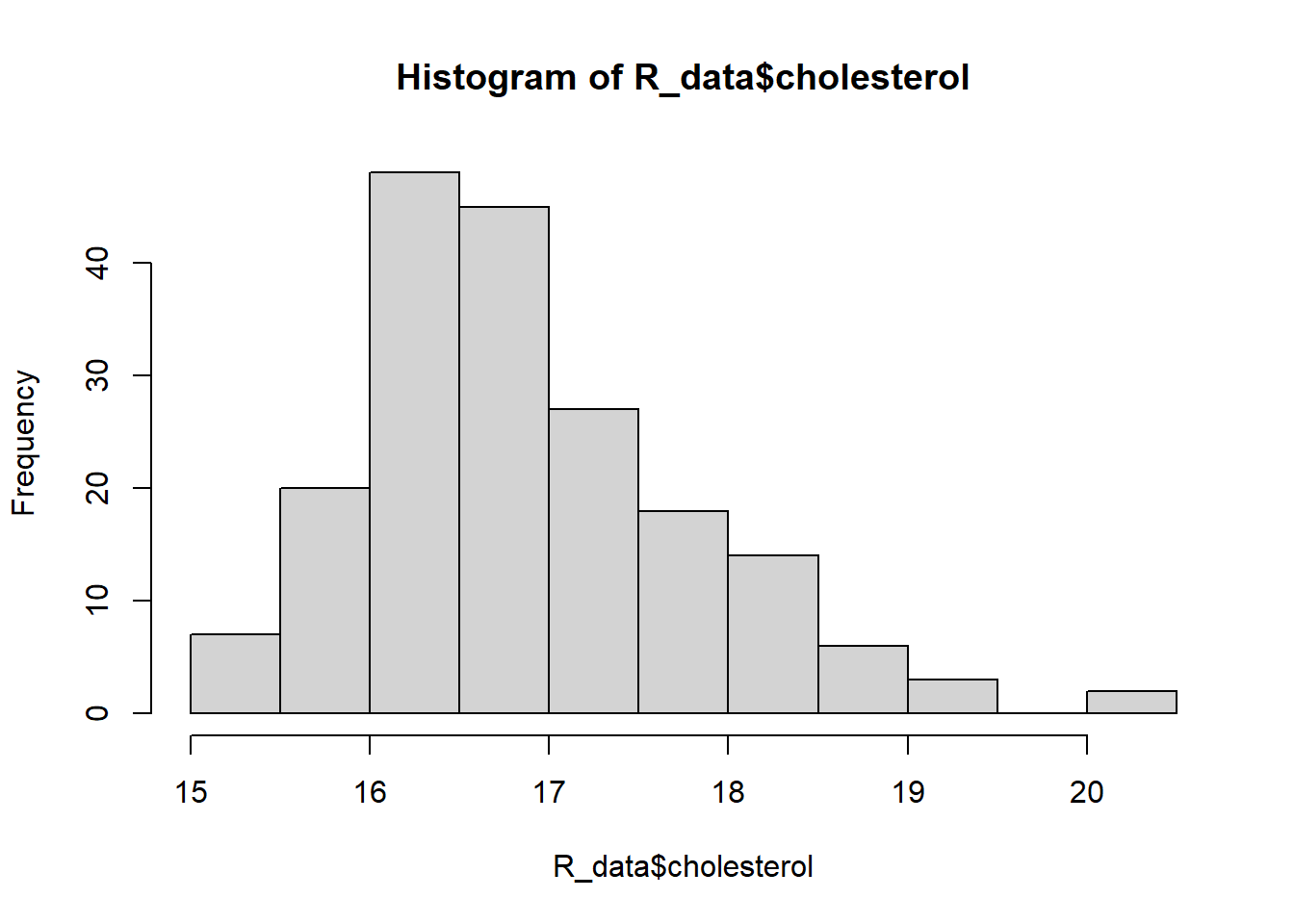
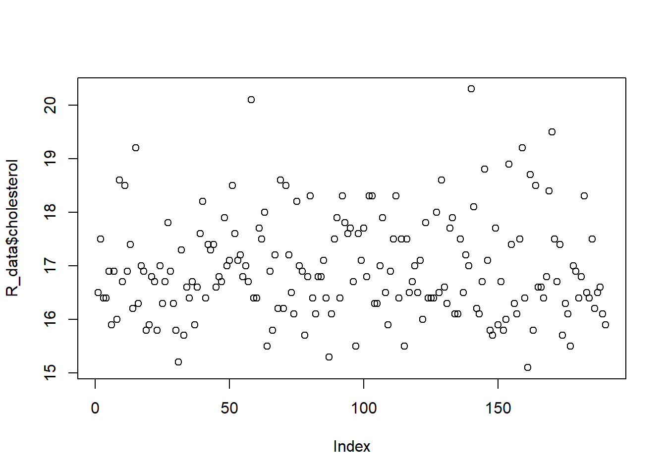
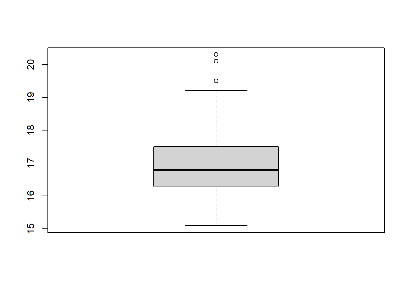
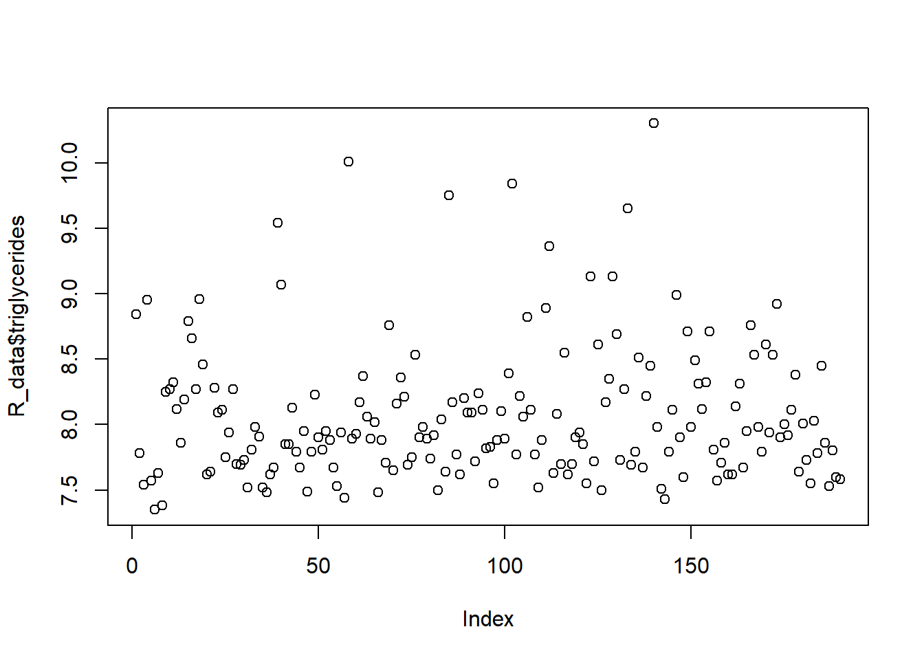
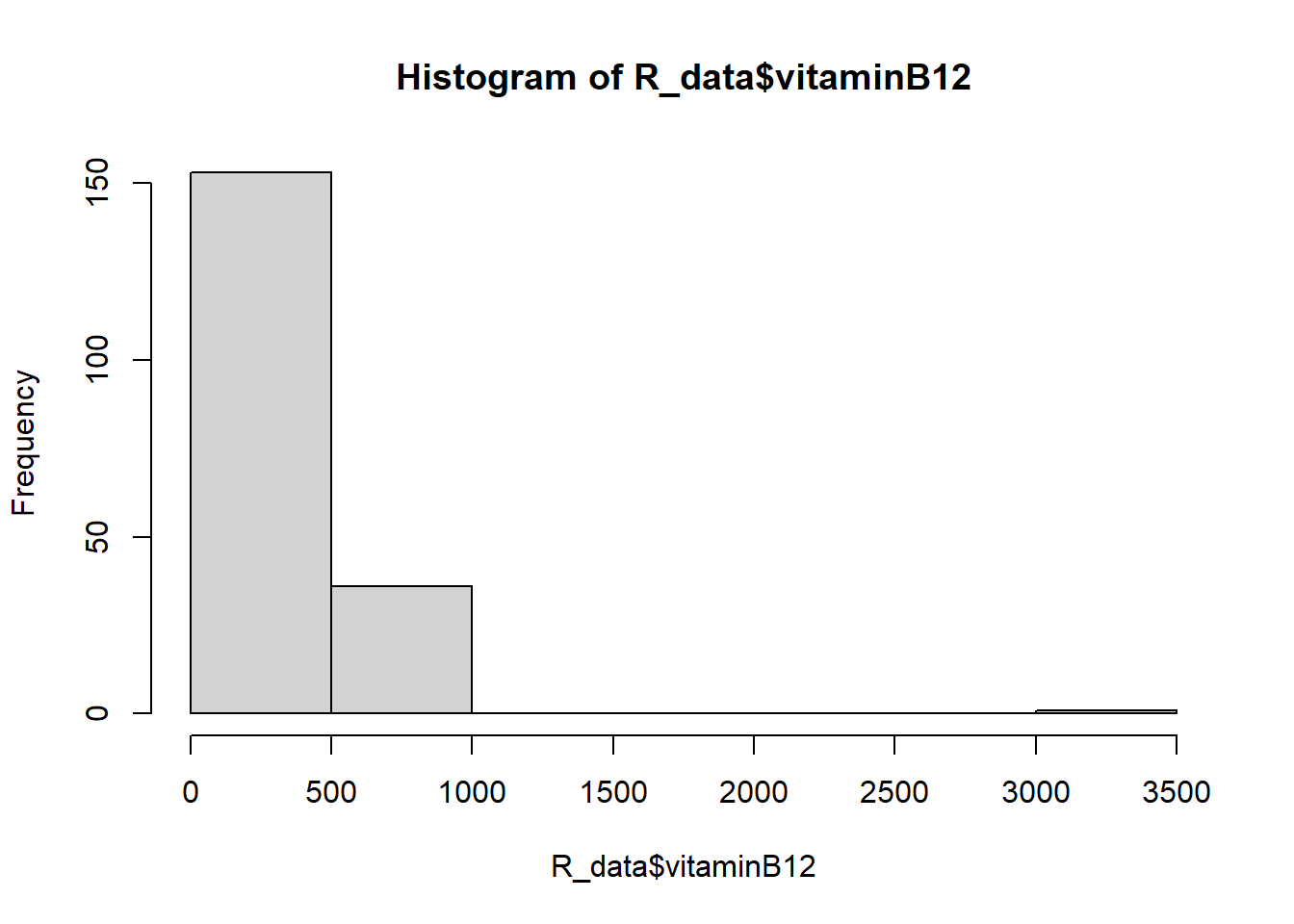
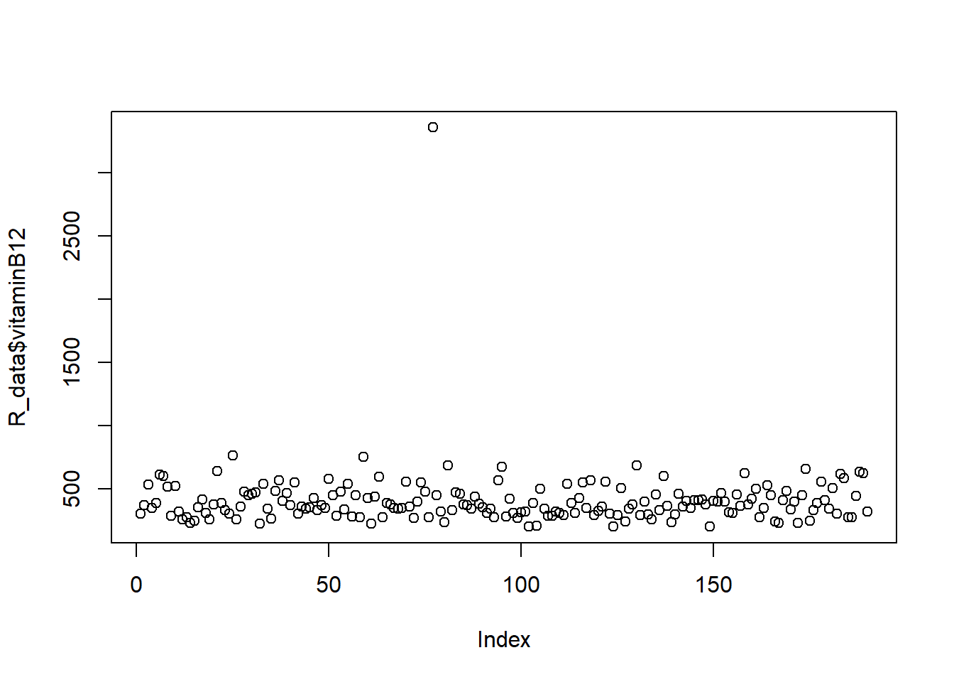
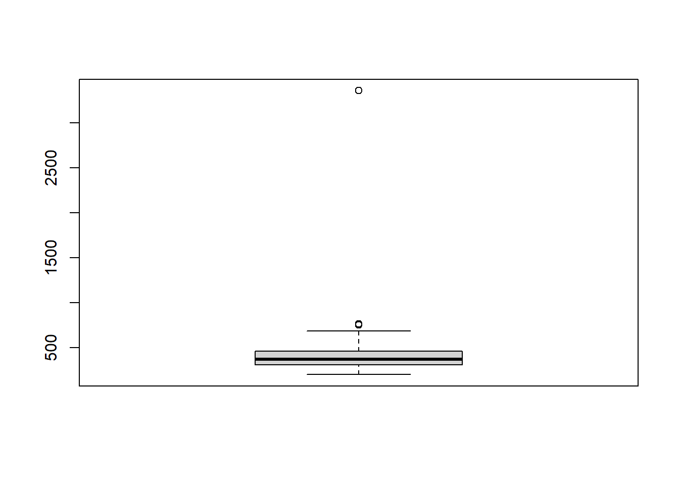
There are several biomarkers collected in the data set. Investigate whether there are outliers in the biomarkers: cholesterol, triglycerides, and vitaminB12. Which functions did you use?

# Cholesterol
hist(R_data$cholesterol)

plot(R_data$cholesterol)

boxplot(R_data$cholesterol)

summary(R_data$cholesterol)
   Min. 1st Qu.  Median    Mean 3rd Qu.    Max. 
  15.10   16.30   16.80   16.94   17.50   20.30 
# triglycerides
hist(R_data$triglycerides)

plot(R_data$triglycerides)

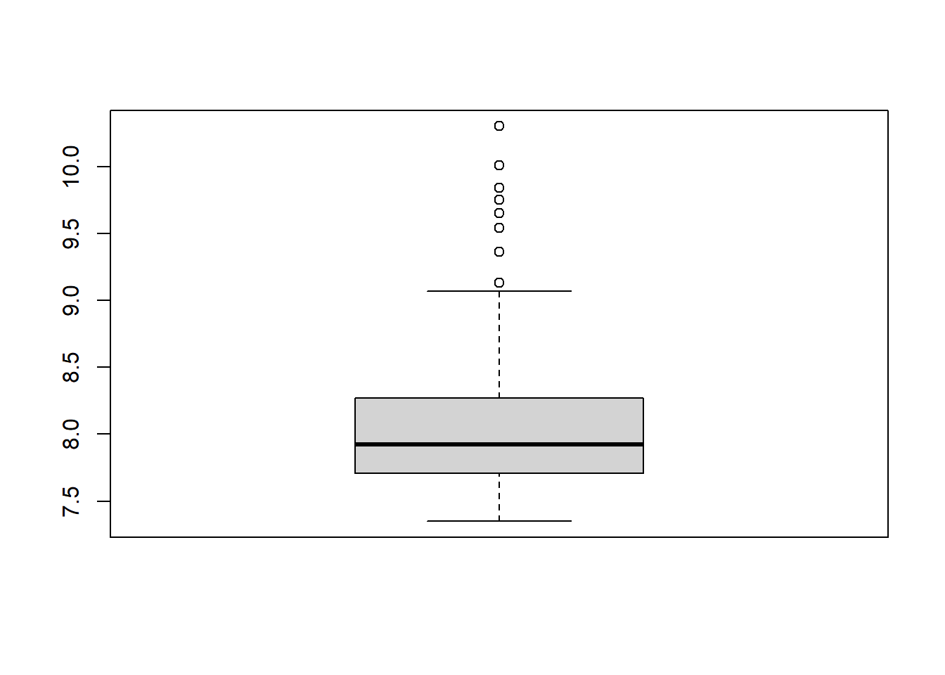
boxplot(R_data$triglycerides)

summary(R_data$triglycerides)
   Min. 1st Qu.  Median    Mean 3rd Qu.    Max. 
  7.350   7.710   7.925   8.068   8.270  10.300 
# vitaminB12
hist(R_data$vitaminB12)

plot(R_data$vitaminB12)

boxplot(R_data$vitaminB12)

summary(R_data$vitaminB12)
   Min. 1st Qu.  Median    Mean 3rd Qu.    Max. 
  201.0   307.0   370.5   409.7   463.0  3360.0 

There is one outlier in vitaminB12.

In question 9 we found an outlier. How do you deal with this outlier?

Knowing that the value of 3360 is an impossible value for vitamin B12, we can decide to remove this measurement. We can either put this measurement to missing (NA)

R_data$vitaminB12_cor <- R_data$vitaminB12
R_data$vitaminB12_cor[R_data$vitaminB12_cor  == 3360] <- NA 
summary(R_data$vitaminB12_cor)
   Min. 1st Qu.  Median    Mean 3rd Qu.    Max.    NA's 
  201.0   307.0   370.0   394.1   463.0   766.0       1 

or we can remove the whole patient

R_data_cor <- R_data[R_data$vitaminB12 != 3360,]
dim(R_data_cor)
[1] 189  25

Fill in the table with summary statistics below

Intellectual disability Normal brain development
(n = …) (n = …)
BMI, median [IQR]
missing (n = )
Educational level Low, n(%)
Intermediate, n(%)
High, n(%)
missing (n = )
Smoking No, n(%)
Yes, n(%)
missing (n = )
SAM, mean (SD)
missing (n = )
SAH, median [IQR]
missing (n = )
Vitamin B12, median [IQR]
missing (n = )

You can change the order of factors

R_data$educational_level <- factor(R_data$educational_level, levels = c('low', 'intermediate', 'high'))

table(R_data$Status)

aggregate(BMI ~ Status, data = R_data, summary)
R_data$educational_level <- factor(R_data$educational_level, levels = c('low', 'intermediate', 'high'))
with(R_data, table(educational_level, Status))
prop.table(with(R_data, table(educational_level, Status)),2)

with(R_data, table(smoking, Status))
prop.table(with(R_data, table(smoking, Status)),2)

aggregate(SAM ~ Status, data = R_data, mean)
aggregate(SAM ~ Status, data = R_data, sd)

aggregate(SAH ~ Status, data = R_data, summary)

aggregate(vitaminB12_cor ~ Status, data = R_data, summary)
Intellectual disability Normal brain development
(n = 82) (n = 108)
BMI, median [IQR] 24 [22 - 27] 24 [22 - 26]
missing (n = 0 )
Educational level Low, n(%) 31 (38%) 14 (13%)
Intermediate, n(%) 34 (41%) 48 (44%)
High, n(%) 17 (21%) 46 (43%)
missing (n = 0)
Smoking No, n(%) 55 (67%) 96 (89%)
Yes, n(%) 27 (33%) 12 (11%)
missing (n = 0)
SAM, mean (SD) 72 (16) 75 (18)
missing (n = 0)
SAH, median [IQR] 16 [15 - 18] 18 [16 - 20]
missing (n = 0)
Vitamin B12, median [IQR] 378 [310 - 477] 363 [305 - 449]
missing (n = 1)