'data.frame':   60 obs. of  3 variables:
 $ len : num  4.2 11.5 7.3 5.8 6.4 10 11.2 11.2 5.2 7 ...
 $ supp: Factor w/ 2 levels "OJ","VC": 2 2 2 2 2 2 2 2 2 2 ...
$ dose: num 0.5 0.5 0.5 0.5 0.5 0.5 0.5 0.5 0.5 0.5 ...R Course - Day 3
Data visualizarion in R
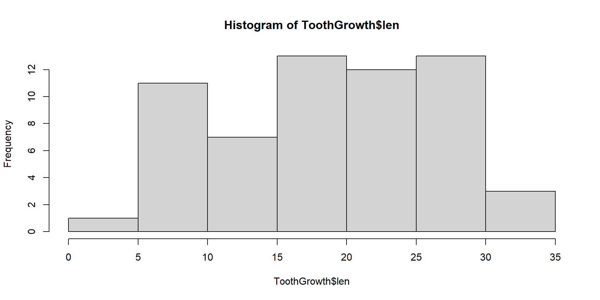
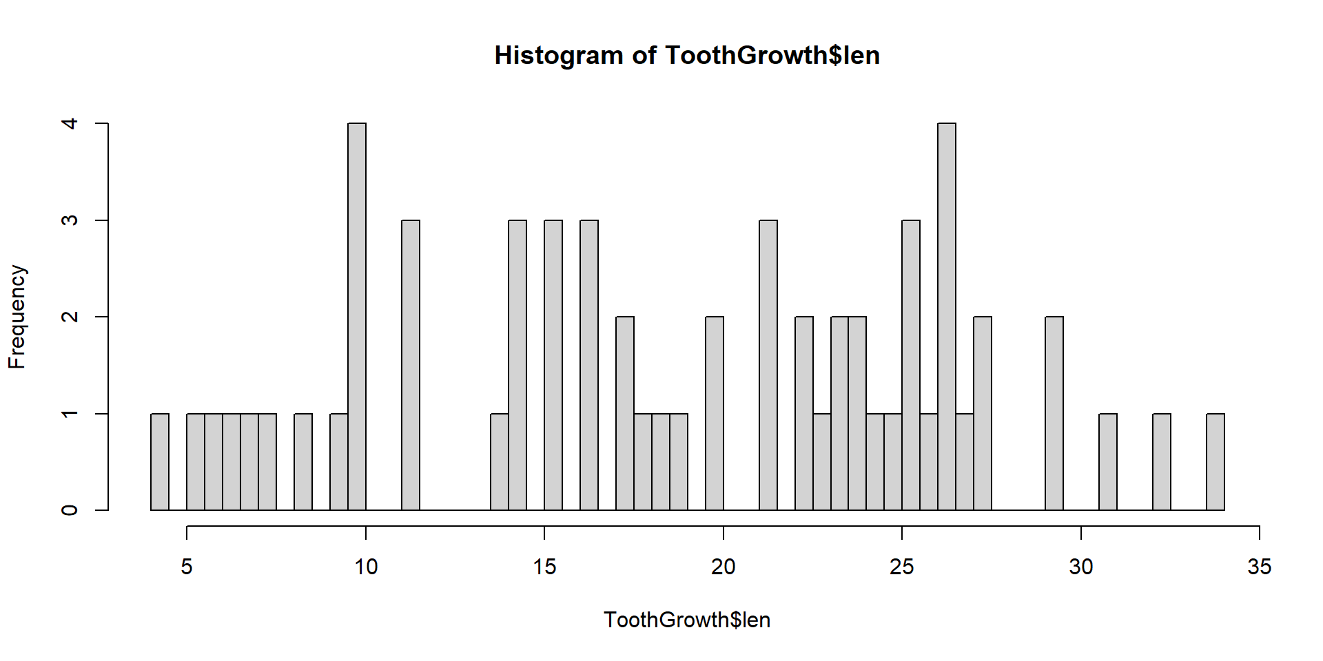
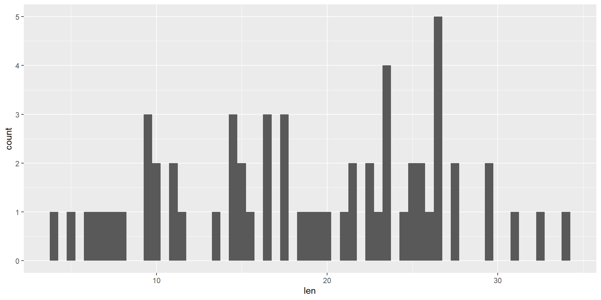
Histograms
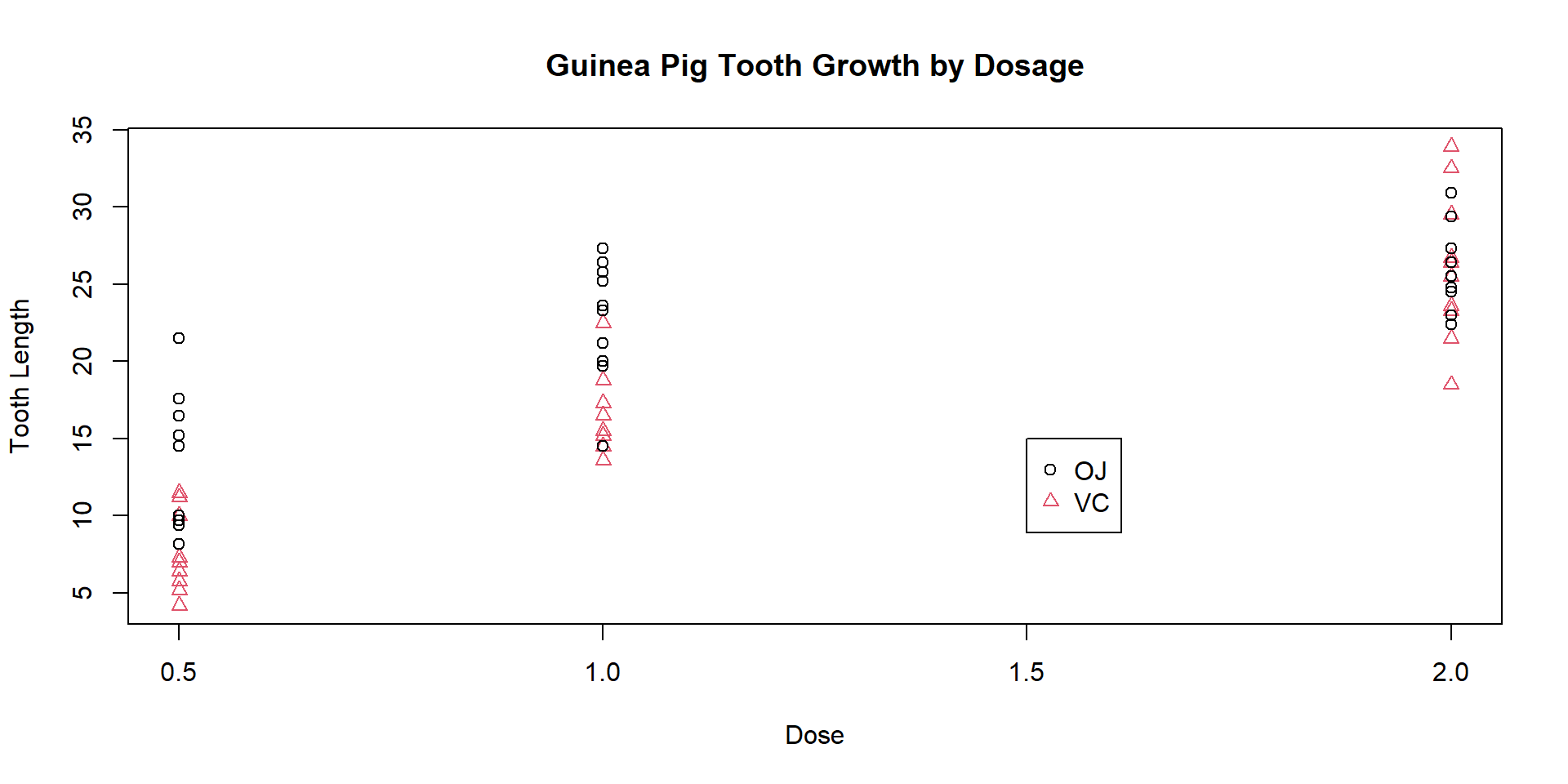
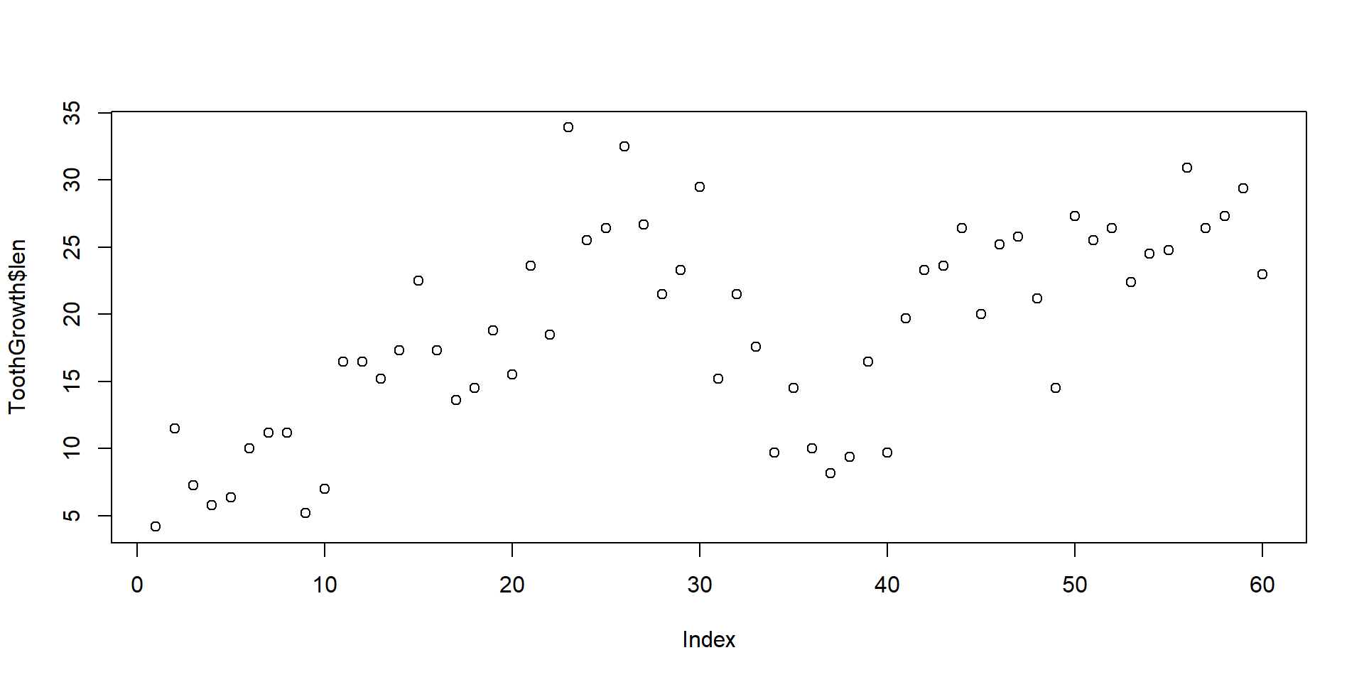
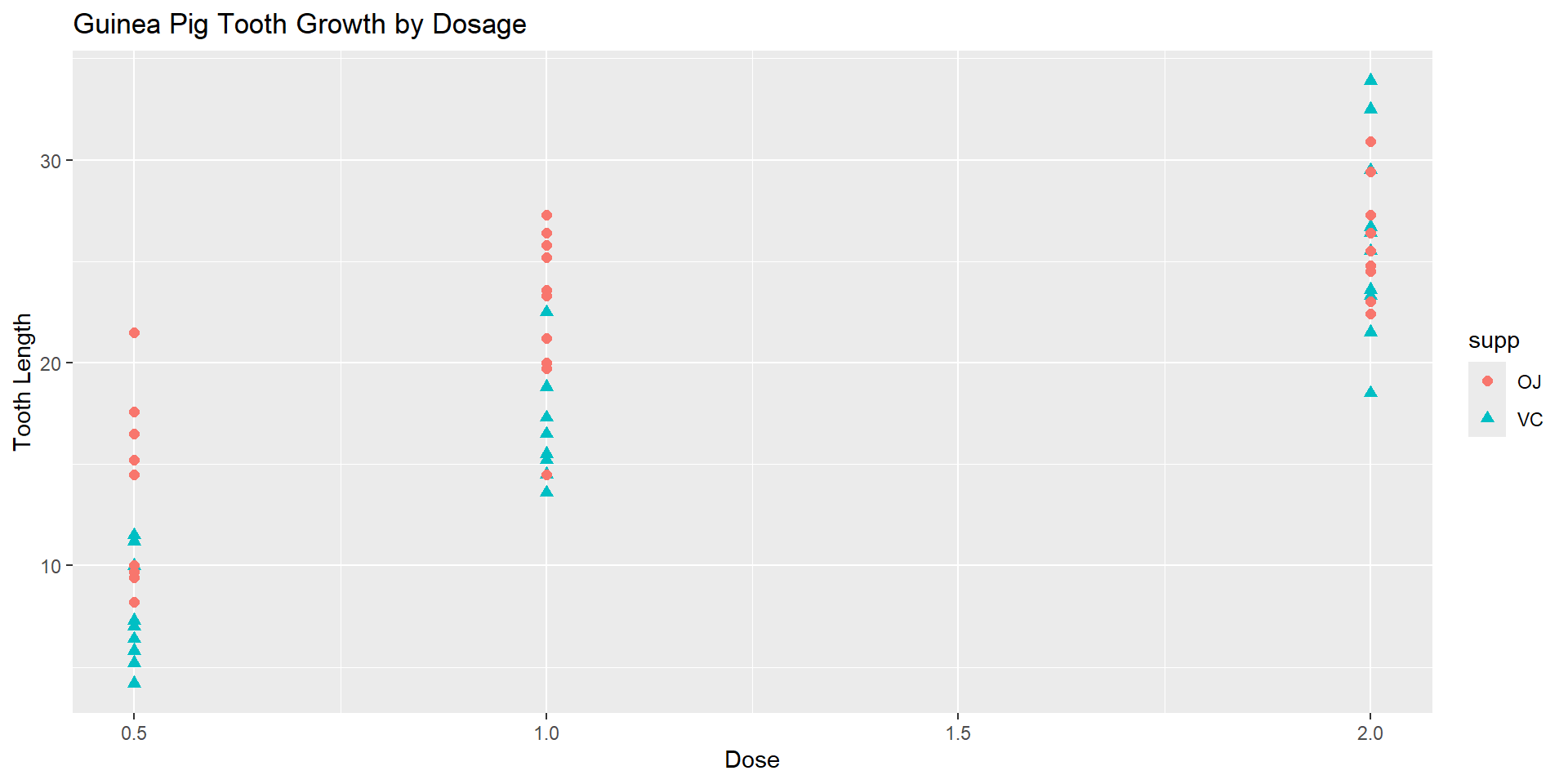
Scatterplots

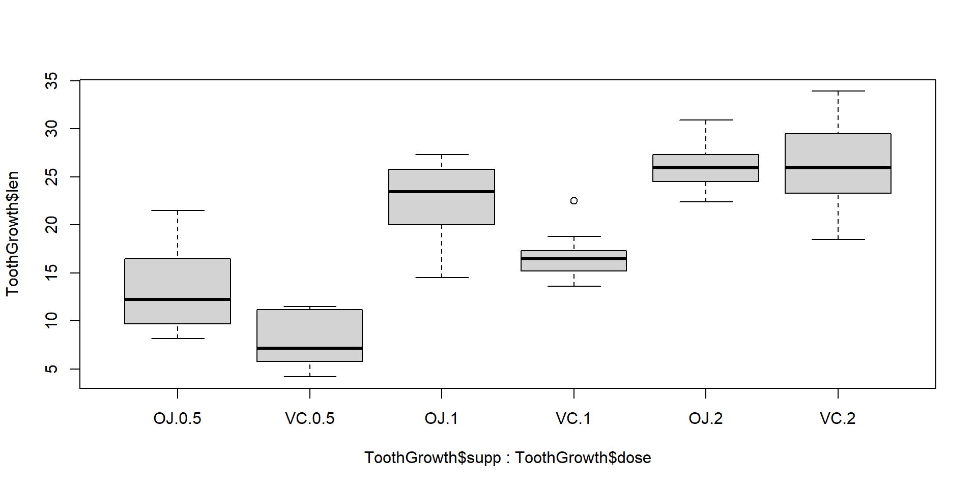
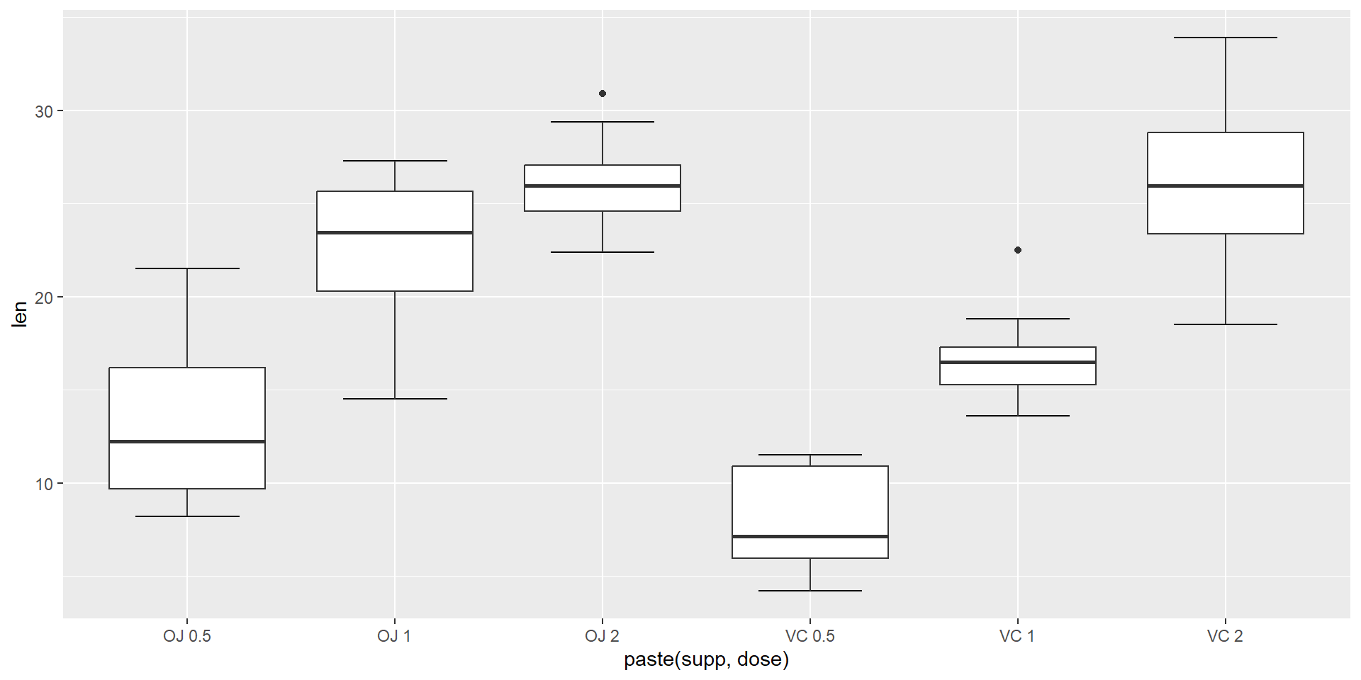
Boxplots
Reformat to One variable One Column
    Deaths Year Month    Sex
1      901 1974   Jan female
2      689 1974   Feb female
3      827 1974   Mar female
4      677 1974   Apr female
5      522 1974   May female
6      406 1974   Jun female
7      441 1974   Jul female
8      393 1974   Aug female
9      387 1974   Sep female
10     582 1974   Oct female
11     578 1974   Nov female
12     666 1974   Dec female
13     830 1975   Jan female
14     752 1975   Feb female
15     785 1975   Mar female
16     664 1975   Apr female
17     467 1975   May female
18     438 1975   Jun female
19     421 1975   Jul female
20     412 1975   Aug female
21     343 1975   Sep female
22     440 1975   Oct female
23     531 1975   Nov female
24     771 1975   Dec female
25     767 1976   Jan female
26    1141 1976   Feb female
27     896 1976   Mar female
28     532 1976   Apr female
29     447 1976   May female
30     420 1976   Jun female
31     376 1976   Jul female
32     330 1976   Aug female
33     357 1976   Sep female
34     445 1976   Oct female
35     546 1976   Nov female
36     764 1976   Dec female
37     862 1977   Jan female
38     660 1977   Feb female
39     663 1977   Mar female
40     643 1977   Apr female
41     502 1977   May female
42     392 1977   Jun female
43     411 1977   Jul female
44     348 1977   Aug female
45     387 1977   Sep female
46     385 1977   Oct female
47     411 1977   Nov female
48     638 1977   Dec female
49     796 1978   Jan female
50     853 1978   Feb female
51     737 1978   Mar female
52     546 1978   Apr female
53     530 1978   May female
54     446 1978   Jun female
55     431 1978   Jul female
56     362 1978   Aug female
57     387 1978   Sep female
58     430 1978   Oct female
59     425 1978   Nov female
60     679 1978   Dec female
61     821 1979   Jan female
62     785 1979   Feb female
63     727 1979   Mar female
64     612 1979   Apr female
65     478 1979   May female
66     429 1979   Jun female
67     405 1979   Jul female
68     379 1979   Aug female
69     393 1979   Sep female
70     411 1979   Oct female
71     487 1979   Nov female
72     574 1979   Dec female
73    2134 1974   Jan   male
74    1863 1974   Feb   male
75    1877 1974   Mar   male
76    1877 1974   Apr   male
77    1492 1974   May   male
78    1249 1974   Jun   male
79    1280 1974   Jul   male
80    1131 1974   Aug   male
81    1209 1974   Sep   male
82    1492 1974   Oct   male
83    1621 1974   Nov   male
84    1846 1974   Dec   male
85    2103 1975   Jan   male
86    2137 1975   Feb   male
87    2153 1975   Mar   male
88    1833 1975   Apr   male
89    1403 1975   May   male
90    1288 1975   Jun   male
91    1186 1975   Jul   male
92    1133 1975   Aug   male
93    1053 1975   Sep   male
94    1347 1975   Oct   male
95    1545 1975   Nov   male
96    2066 1975   Dec   male
97    2020 1976   Jan   male
98    2750 1976   Feb   male
99    2283 1976   Mar   male
100   1479 1976   Apr   male
101   1189 1976   May   male
102   1160 1976   Jun   male
103   1113 1976   Jul   male
104    970 1976   Aug   male
105    999 1976   Sep   male
106   1208 1976   Oct   male
107   1467 1976   Nov   male
108   2059 1976   Dec   male
109   2240 1977   Jan   male
110   1634 1977   Feb   male
111   1722 1977   Mar   male
112   1801 1977   Apr   male
113   1246 1977   May   male
114   1162 1977   Jun   male
115   1087 1977   Jul   male
116   1013 1977   Aug   male
117    959 1977   Sep   male
118   1179 1977   Oct   male
119   1229 1977   Nov   male
120   1655 1977   Dec   male
121   2019 1978   Jan   male
122   2284 1978   Feb   male
123   1942 1978   Mar   male
124   1423 1978   Apr   male
125   1340 1978   May   male
126   1187 1978   Jun   male
127   1098 1978   Jul   male
128   1004 1978   Aug   male
129    970 1978   Sep   male
130   1140 1978   Oct   male
131   1110 1978   Nov   male
132   1812 1978   Dec   male
133   2263 1979   Jan   male
134   1820 1979   Feb   male
135   1846 1979   Mar   male
136   1531 1979   Apr   male
137   1215 1979   May   male
138   1075 1979   Jun   male
139   1056 1979   Jul   male
140    975 1979   Aug   male
141    940 1979   Sep   male
142   1081 1979   Oct   male
143   1294 1979   Nov   male
144   1341 1979   Dec   male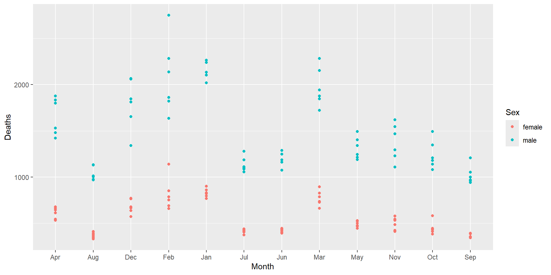
Geometries
geom_… - the thing you want to plot
30+ different geoms: https://ggplot2.tidyverse.org/reference/
geom_point()![]()
geom_line()![]()
geom_bar()![]()
geom_histogram()![]()
geom_boxplot()![]()
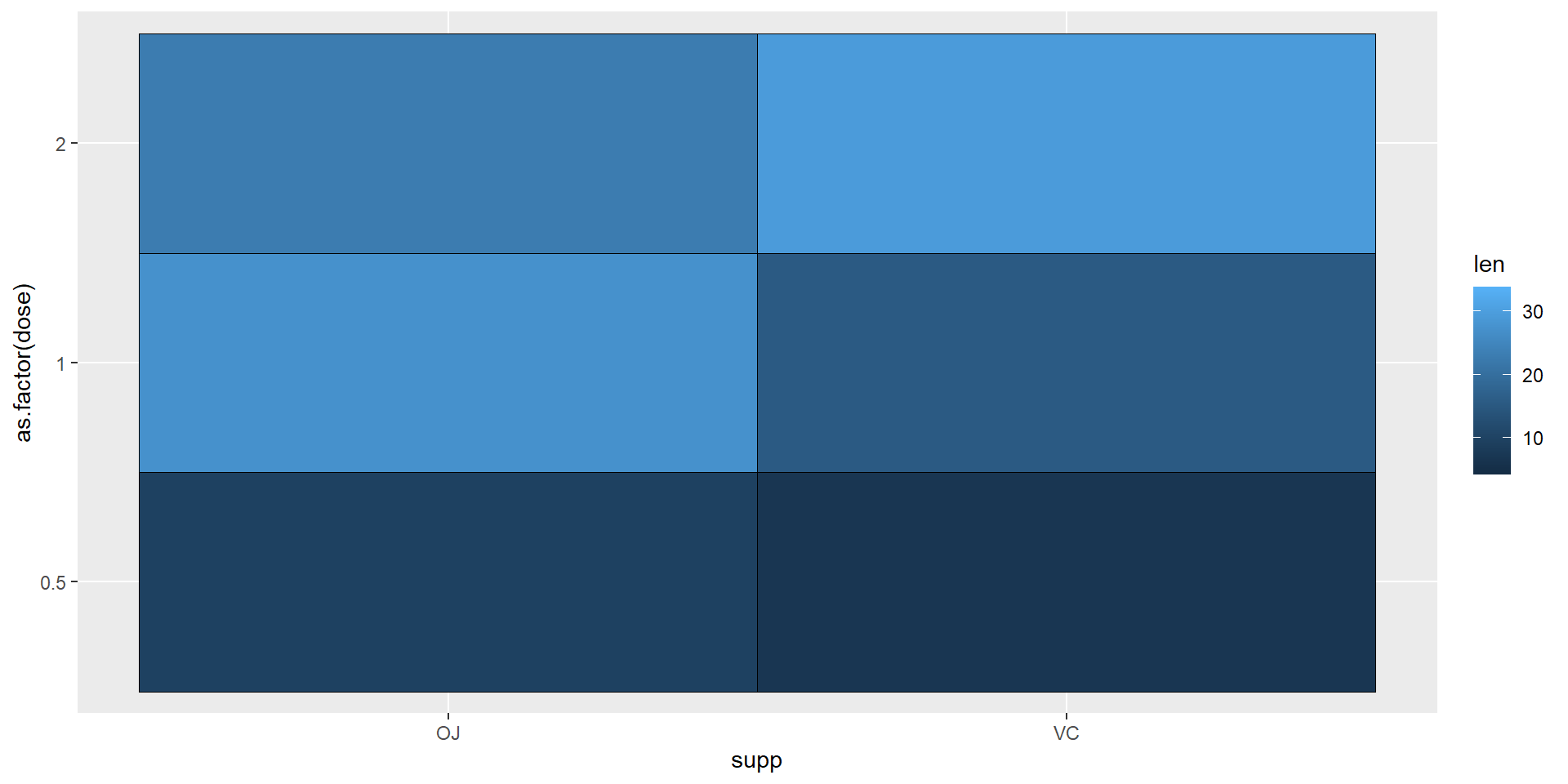
geom_heatmap()![]()
Scatter Plots
Histograms
Box Plots

Heatmaps
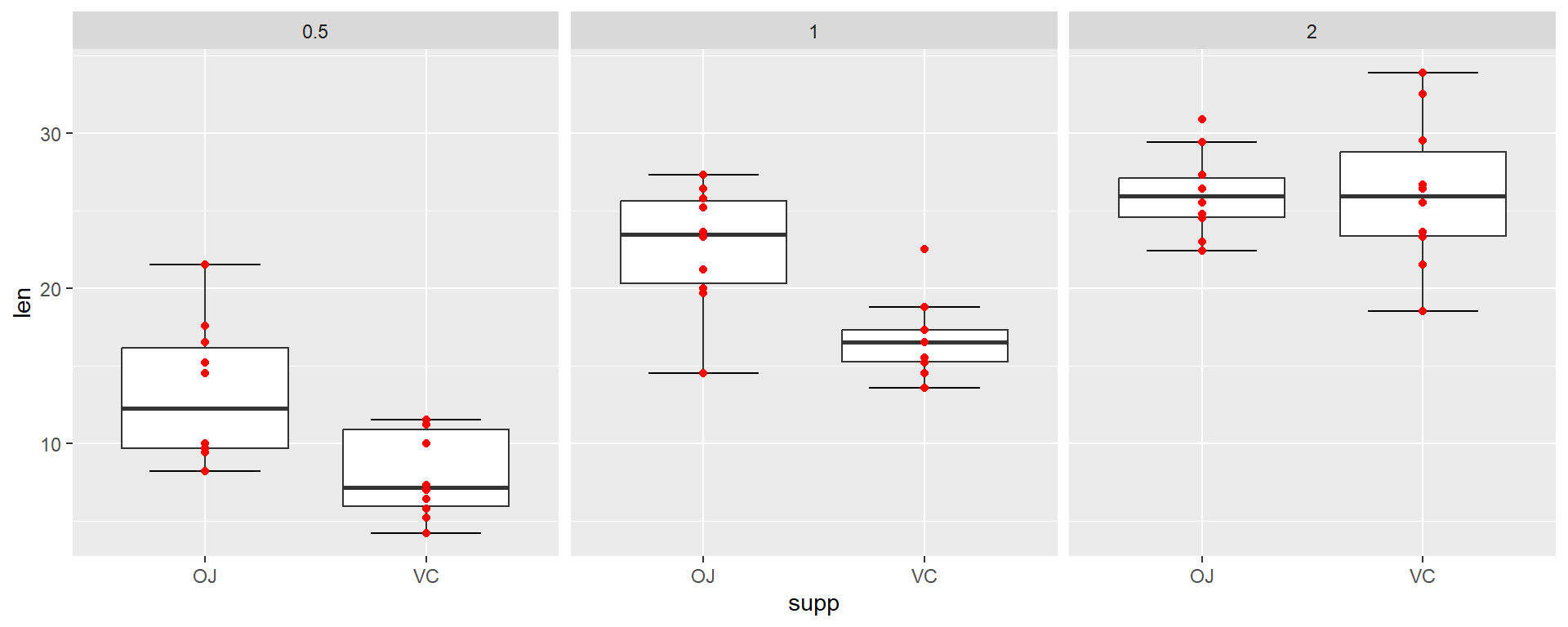
Facets
Separate plots (facets) to compare groups of data
par(mfrow = c(1, 3))
low <- ToothGrowth[which(ToothGrowth$dose==0.5),]; boxplot(low$len~low$supp, main = "Low dose", xlab = "Supplement Type")
med <- ToothGrowth[which(ToothGrowth$dose==1),]; boxplot(med$len~med$supp, main = "Medium dose", xlab = "Supplement Type")
high <- ToothGrowth[which(ToothGrowth$dose==2),]; boxplot(high$len~high$supp, main = "High dose", xlab = "Supplement Type")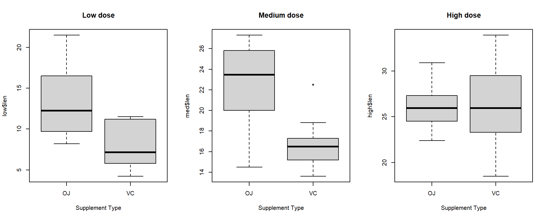
Scales
Scale can be changed for each Aesthetic with corresponding scale_...
ggplot(ToothGrowth, aes(x=index, y=as.factor(dose), color=len)) +
    geom_point() +
    scale_x_continuous(limits=c(1,100), trans = "log2",
        breaks=c(2,4,8,16,32,64),
        label=c("two","four","eight","sixteen","thirtytwo","sixtyfour")) +
    scale_y_discrete(label=c("low","medium","high")) +
    scale_color_gradient2(limits=c(0,40), low = "green", mid = "black", high = "red",
        midpoint = 20)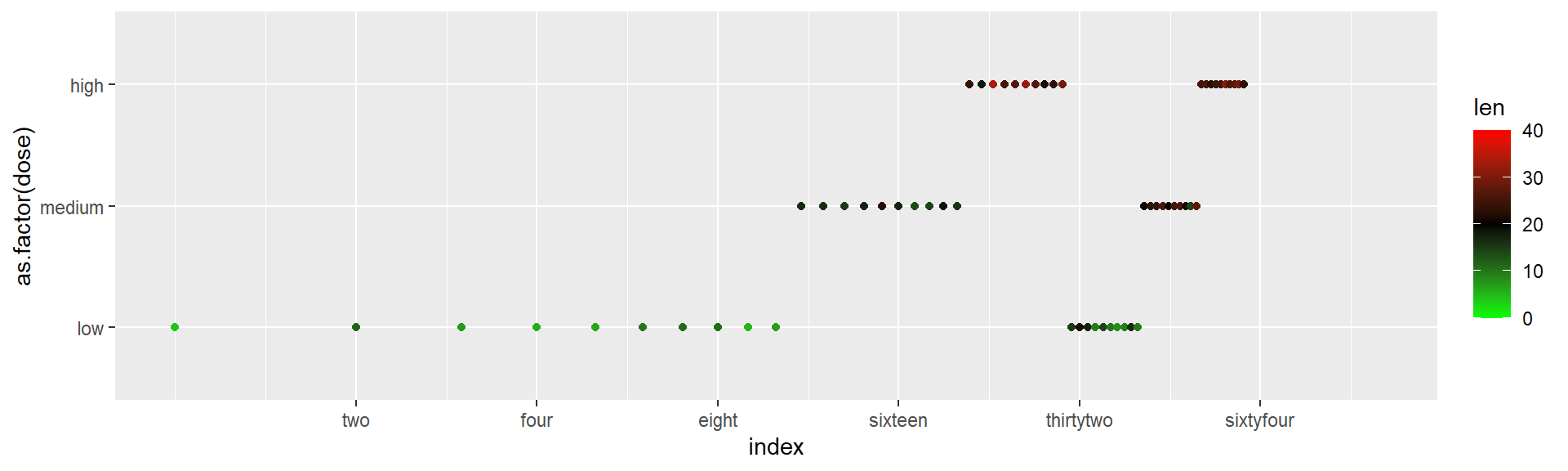
All available scales with examples: http://ggplot2.tidyverse.org/reference/
Themes
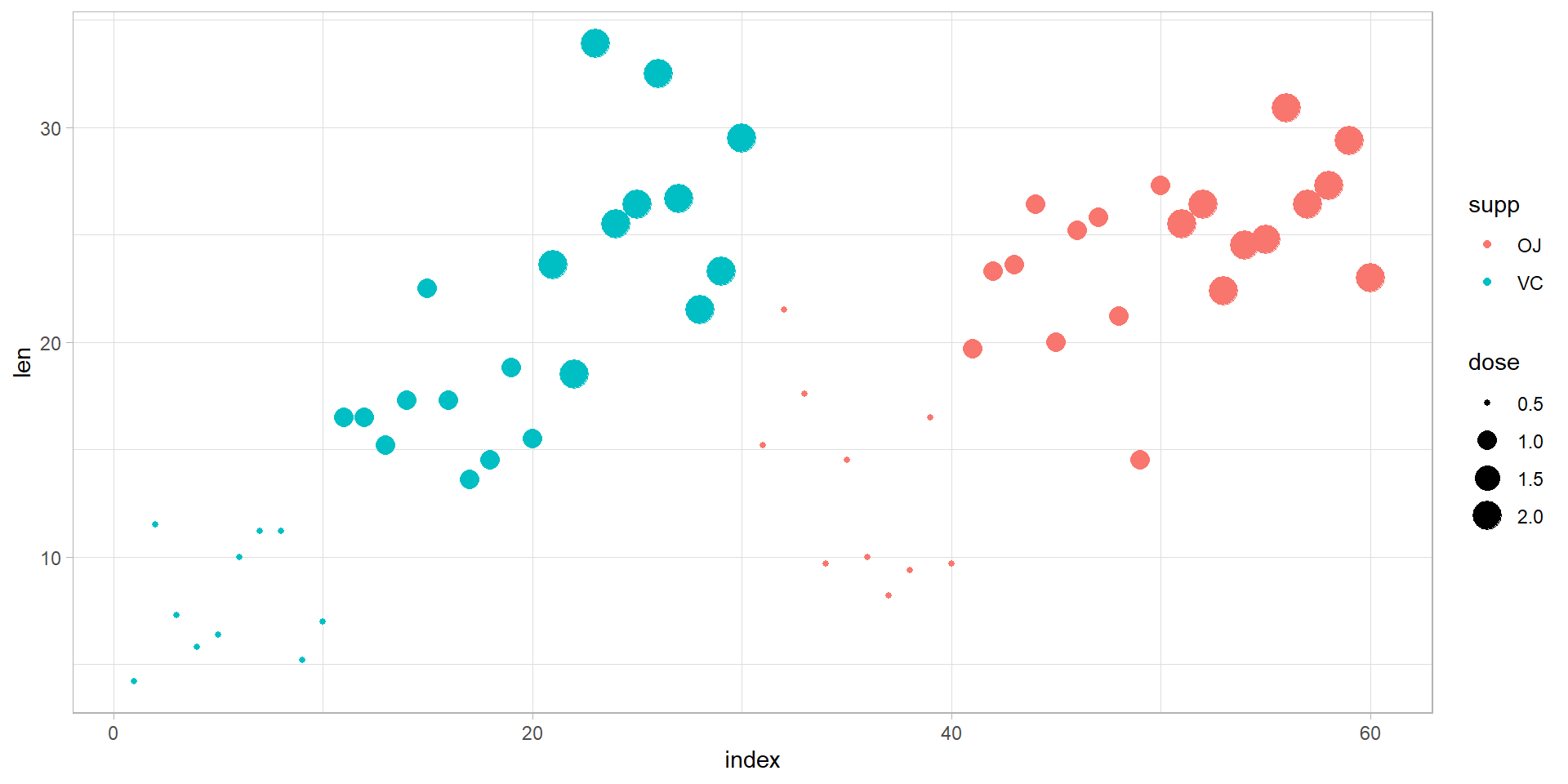
Custom Themes
Theme parameters: http://ggplot2.tidyverse.org/reference/theme.html
Customize labels with labs()
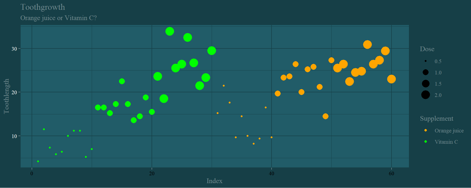
p <- ggplot(ToothGrowth)
p + geom_point(aes(x = index, y = len, color = supp, size = dose)) +
    theme(text = element_text(family = "serif", colour = "#6f898e"),
      line = element_line(color = "#163f47"),
      rect = element_rect(fill = "#163f47", color = "#163f47"),
        axis.text.x = element_text(color="black"),
        axis.text.y = element_text(color="white"),
      axis.ticks = element_line(color = "#6f898e"),
      axis.line = element_line(color = "#163f47", linetype = 1),
        legend.background = element_blank(),
        legend.key = element_blank(),
        panel.background = element_rect(fill = "#215c68", colour = "#163f47"),
        panel.border = element_blank(),
      panel.grid = element_line(color = "#163f47"),
      panel.grid.major = element_line(color = "#163f47"),
      panel.grid.minor = element_line(color = "#163f47"),
      plot.background = element_rect(fill = NULL, colour = NA, linetype = 0)
    ) +
    labs(title="Toothgrowth",
        subtitle = "Orange juice or Vitamin C?", x="Index", y="Toothlength",
        size="Dose", color="Supplement") +
    scale_color_manual(label=c("Orange juice","Vitamin C"),
        values = c("VC"="green","OJ"="orange"))